User Guide
Everything about using OpticSketcher on desktop or tablet, from placing your first lens to building complete optical systems and sharing them with others.
Getting Started: Your First Optical System
This five-minute walkthrough builds a classic focusing setup: a collimated laser beam passing through a lens and landing on a sensor. No account is needed, so just open the workspace and follow along.
Interface Overview
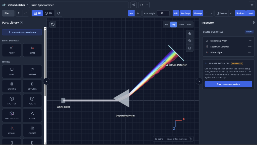
The workspace is built around a live 3D canvas with a parts library on the left and an inspector on the right. Everything updates in real time; there is no separate "simulate" step.
 12345
12345The top toolbar in detail
- File menu: new design, Examples (classic systems and tutorials loaded into the workspace), save / load a local .json file, import Zemax .zmx or OpTaliX .otx, export (PNG, SVG, OBJ, STL, PLY, GLB, ZMX), and Help (What’s new, quick guide, About).
- Project name: click to rename; the name is used for cloud saves, share links and exported file names.
- Undo / Redo: step back and forward through every edit (Ctrl/Cmd + Z / Ctrl/Cmd + Shift + Z).
- 2D / 3D: switch between a flat schematic-style view and a full 3D perspective view of the same scene.
- Units (mm / in): every numeric field in the app switches between millimeters and inches.
- Axis Height: the global optical-axis height; new elements are placed at this height so systems stay aligned.
- Grid & Pos Snap: show / hide the grid and snap element positions to it while dragging.
- Rays: show or hide the traced rays without changing the design. Use this for a cleaner look at the hardware; the simulation still runs.
- Live rays + angle snap: toggle continuous ray tracing while dragging, and choose the rotation snap increment (e.g. 1°) used by rotation handles and angle sliders. This is separate from the Rays visibility toggle.
- Section: cut the scene with a clipping plane to look inside thick glass elements.
- Shadows / Labels: toggle rendered shadows and floating element name labels.
- Share & Cloud: generate share links and save designs to your cloud account (see Files, Cloud & Sharing).
- Theme: switch between dark and light workspace themes.
Panels
- Parts Library (left): all sources, optics and sensors, plus the AI Scene Assistant. Collapse or open it with the round arrow button on the left edge of the canvas.
- Inspector (right): when nothing is selected it shows the Scene Overview tree (click any row to select that element, expand groups with the arrow) and the AI system analysis. When an element is selected it shows every editable property of that element. Toggle the panel with the round arrow on the right edge.
- Mode hint: the small "i" chip at the bottom of the canvas summarizes what the mouse buttons do in the current view mode; hover it for the full list.
- Help: the round "?" button on the canvas opens the built-in quick guide. File → What’s new lists product changes since your last visit (returning users only; first-time visitors are not interrupted).
Adding & Editing Parts
Adding parts
- Click a part in the library: a new instance is placed at the default workspace position and selected.
- Drag a part from the library onto the canvas: the preview follows the pointer and drops exactly where you release.
- Custom meshes: the custom mirror, prism and beam-blocker entries can import your own geometry from .obj, .stl or .ply files, which then behave as real optical elements in the ray trace.
Selecting
- Click an element to select it; click empty space to deselect.
- Shift + click: add or remove elements from the selection.
- Shift + right-drag: box (marquee) selection of everything inside the rectangle.
- Ctrl/Cmd + A: select all elements.
- Click a row in the Scene Overview tree (Inspector) to select that element, useful in crowded scenes.
Moving & rotating
- Drag a selected element to move it. With Pos Snap on, it snaps to the grid.
- Shift + drag: constrain movement to a single axis.
- Drag the circular rotation ring around a selected element to rotate it; rotation snaps to the angle increment chosen in the toolbar.
- Arrow keys: nudge the selection in small steps for precise placement.
- For exact values, type position and rotation (pitch / yaw / roll) directly in the Inspector.
Visibility & labels
- Show object in the Inspector hides the part on the canvas; it stays in the scene list so you can select it again.
- Show label hides just the floating name. You can pin the label above, below, left or right, or drag it on the canvas to a clearer spot.
Editing properties
Every element type has its own set of Inspector controls. For example, a lens Construction is Thin (ideal focal length only), Singlet (radii, thickness, glass, and a bending slider that keeps power while changing form), or Cemented doublet (two glasses, three surfaces, no air gap). Spherical or cylindrical applies to all three. A source exposes wavelength (with a live color preview) - enter one value, or several comma-separated wavelengths such as450, 532, 633 to launch those lines at once - plus ray count, beam width, divergence and polarization. Changes apply instantly to the ray trace.
Groups & locking
- Ctrl/Cmd + G groups the selection so it moves and rotates as one unit (e.g. a multi-element objective); Ctrl/Cmd + Shift + G ungroups. Groups appear as expandable folders in the scene tree.
- Lock prevents an element from being moved or rotated on the canvas, handy for reference elements you don't want to disturb. Lock and unlock from the context menu or Inspector.
Copy, paste & duplicate
- Ctrl/Cmd + D: duplicate the selection in place (with a small offset).
- Ctrl/Cmd + C / X / V: copy, cut and paste through the system clipboard. The clipboard uses structured JSON, so you can copy elements in one browser tab and paste them into a different design in another tab.
- All of these are also available in the right-click context menu on the canvas.
Keyboard Shortcuts
Shortcuts are ignored while your cursor is inside a text field or numeric input. On Mac, use Cmd instead of Ctrl.
| Shortcut | Action |
|---|---|
| Delete / Backspace | Delete the current selection. |
| Ctrl + A | Select all elements. |
| Ctrl + D | Duplicate the selection (with a small offset). |
| Ctrl + Z | Undo the last edit. |
| Ctrl + Shift + Z / Ctrl + Y | Redo. |
| Ctrl + G | Group the selection. |
| Ctrl + Shift + G | Ungroup the selected group. |
| Ctrl + C | Copy the selection to the system clipboard (structured JSON; works across browser tabs). |
| Ctrl + X | Cut: copy to the clipboard, then remove from the scene. |
| Ctrl + V | Paste from the clipboard. Pasted items get new IDs and a small offset. Also accepts a plain JSON array in the saved-design format, and a URL to a .zmx lens file (e.g. a Thorlabs link), which triggers a direct ZMX import. |
| Arrow keys | Nudge the selection in small steps. |
| Shift (held while dragging) | Constrain movement to one axis. |
| Esc | Close open dialogs. |
Views & Display Options
2D vs 3D
The 2D mode renders the scene as a flat, schematic-style drawing, ideal for classic optical-bench layouts and publication figures. The 3D mode shows the same scene with full perspective, shadows and depth, which matters for systems with out-of-plane folds or cylindrical optics. Switching modes never changes your design, only how it's drawn.
View presets
The floating strip at the top-right offers Iso (isometric), Top, Front and Side orthographic presets, plus zoom in / out and a home button that resets the camera to fit the whole scene. In flat presets (Top / Front / Side), dragging on empty space pans; in Iso and 3D it orbits.
Display toggles (toolbar)
- Grid: show or hide the reference grid.
- Pos Snap: snap dragged elements to the grid.
- Rays: show or hide traced rays on the canvas without changing the design.
- Live rays: keep tracing rays continuously while you drag; the adjacent dropdown sets the rotation snap angle (e.g. 1°). This is separate from Rays visibility.
- Section: enable a clipping plane that cuts the scene open, letting you see ray paths inside thick lenses and prisms. The adjacent dropdown selects the cut plane.
- Shadows: toggle rendered shadows in 3D.
- Labels: show or hide floating element name labels on the canvas.
- Axis Height: the global optical-axis height (all new parts are placed at this height).
- mm / in: switch every field in the app between metric and imperial units.
- Theme: dark or light workspace (the sun / moon button at the top-right).
Files, Cloud & Sharing
Local files
The File menu saves your design as a local .json file and loads it back later: a fully self-contained snapshot you can keep, version or email. Guests (without an account) can work entirely with local files; the current sketch is also kept in the browser between visits.
Examples
File → Examples lists classic forms and tutorials from the same library as the public Gallery. Choosing one replaces the current sketch (you will be asked to confirm if you have unsaved work) so you can explore a working system immediately.
Cloud designs
- Sign in and use the cloud button in the toolbar to save designs to your account and open them from any device.
- Each design keeps a revision counter: if the same design was changed on another device, you'll get a conflict prompt instead of silently overwriting your work.
- The cloud picker shows a thumbnail preview of every saved design.
Sharing
- Temporary link: a self-contained snapshot of the current design; anyone with the link can open it for 14 days. No account needed on either side.
- Permanent link: linked to a cloud design; it always opens the latest saved version and never expires. Requires the design to be saved to the cloud.
Import & export formats
| Format | Direction | What it does |
|---|---|---|
| .json | Save / Load | Native design file: full scene, lossless. |
| .zmx | Import / Export | Zemax sequential lens prescriptions. Import from a file, or simply paste a public ZMX URL (e.g. a Thorlabs product link) onto the canvas with Ctrl+V or the right-click menu. Export converts lens stacks on a straight axis back to ZMX. |
| .otx | Import | Optional OpTaliX / CODE V-style sequential file (rdy/thi/gla or S lines). Use this if you already have Handbook of Optical Systems designs — OpticSketcher does not bundle those ~339 files. Convert in OpTaliX-LT to ZMX if a command is not recognized. |
| .obj / .stl / .ply | Import / Export | Import custom meshes as mirrors, prisms or blockers; export the whole scene (or the selection) as solid geometry for CAD. |
| .glb | Export | 3D scene export for viewers and rendering tools. |
| .png / .svg | Export | Publication-ready images of the current view; SVG stays crisp at any scale. |
| .csv | Export | Sensor hit data (position, intensity, wavelength, polarization) from the sensor analysis window. |
Embedding a Design on a Website
Any design can be published as a live, ray-traced viewport inside another page - a lecture site, a lab wiki, a product page or a blog post. Visitors see the real simulation, not a screenshot: the same engine, the same optics and the same rays as in the editor, with only the interaction limited to what you allow.
Creating the embed code
Interaction modes
| Mode | What visitors can do |
|---|---|
| Static view | Nothing - a live-rendered but fixed diagram. Best for figures inside text. |
| Camera only | Rotate, pan and zoom the scene. The optics themselves cannot be moved. |
| Draggable parts | Move the parts you name, optionally locked to a single axis. Everything else stays fixed. |
In "Draggable parts" mode the generator lists every part in your design. Tick the ones a visitor may move, and choose Free, X only or Z only for each - an axis lock keeps a lens on the optical axis while still letting the visitor explore focus.
Parametric sliders
Sliders turn an embed into a teaching demo, and each slider is bound to one parameter of one specific part. The generator lists the parts in your design and, under each, exactly the parameters that part can expose: focal length or the two curvature radii of a lens, the radius of a spherical mirror, the yaw, pitch and roll of a prism or mirror, refractive index, wavelength, divergence, split ratio, polarizer or waveplate axis, Faraday rotation, grating density and more.
The rays retrace live as the visitor moves a slider, so a single embed can show how the image distance follows the focal length, how dispersion through a rotating prism changes with wavelength, or how a curvature change turns a collimated beam into a focus.
AI Tools & Sensor Analysis
AI Scene Assistant
The button at the top of the Parts Library opens the AI scene assistant. Describe what you want in plain language - for example "a Keplerian telescope with 200 mm and 50 mm lenses", "set the lens focal length to 150 mm", "delete the prism", or "move the sensor to x=400". The assistant can add new parts, update pose or properties of existing elements, and delete elements you ask to remove. Changes are validated with the ray tracer before they are applied as a single undoable step, and everything remains fully editable afterwards. If something is selected on the canvas, the assistant prefers those elements when you say "this" or "the selected".
After a generation, you can ask for a revision of the last AI-added batch ("Request a fix"), or remove elements that session added. Always verify positions, orientations, and the traced rays.
Named classic designs (Cooke, Tessar, Planar, Distagon, Plössl, Cassegrain, and many Handbook-style aliases) are recognized by name, type, description and parameters. The assistant maps them onto a curated scalable form — it does not load the commercial ~339 HOS files. If EFL, F/# or object distance is missing or several names match, it asks a short clarifying question first. To place an exact OpTaliX prescription you already own, use File → Import OpTaliX (.otx).
Analyze current system (AI)
In the Inspector (with nothing selected), Analyze current system asks the AI to explain what your setup does: where the light goes, what each element contributes, and what the system as a whole achieves. You can ask follow-up questions. This feature is experimental: always verify its conclusions against the traced rays. Analysis does not change the scene - use the Scene Assistant to edit.
Sensor analysis window
- Select a sensor and open its captured hits from the Inspector to see a spot diagram: a 2D scatter of every ray hit on the sensor face, colored by true wavelength, with pan and zoom.
- The statistics tab shows intensity-weighted centroid and spread, wavelength distribution, degree of polarization (DoP) and Stokes parameters.
- The hits table lists each individual ray with its position, intensity, wavelength and polarization state.
- Export the plot as an image or the raw data as CSV for further analysis.
Parts Reference
Light sources
| Part | What it does |
|---|---|
| Point Source | Emits diverging rays from a single point over an adjustable cone angle. Models LEDs, fiber tips and point emitters. Wavelength (one value, or several comma-separated nm values), ray count and polarization are adjustable. |
| Collimated Beam | Parallel bundle of rays with adjustable width, ray count, wavelength (one value, several comma-separated nm values, or white light) and polarization. Models lasers and collimated illumination. Gaussian intensity profile supported. |
Optics
| Part | What it does |
|---|---|
| Lens | Refractive lens with spherical, cylindrical, parabolic or aspheric surfaces (conic constant + higher-order terms). Construction: Thin, Singlet, or Cemented doublet (switching forms keeps focal length). Thin is an ideal lens defined only by focal length. A doublet is two glasses in contact (front, shared cement radius, rear) with no air gap; it can be spherical or cylindrical. Set focal length or radii, diameter, thickness (or two glass thicknesses), and glass from a real material catalog (including optical plastics). Cylindrical lenses focus in one axis; rotate (roll 90°) to switch the active axis. Spherical singlets have a bending slider that keeps focal length while changing shape. Catalog doublet pairs: N-BK7/N-SF2, N-SK16/F2, PMMA/PC. |
| Mirror | Flat, spherical or parabolic reflector, round or rectangular, with optional custom mesh geometry. Curved mirrors focus or expand beams like in reflective telescopes. |
| Beamsplitter | Cube splitter that divides each ray into transmitted and reflected parts by an adjustable ratio. |
| Polarizing BS | Polarizing beamsplitter cube. Transmits p-polarization and reflects s-polarization, splitting by polarization state. |
| Spectral Splitter | Dichroic-style cube that routes rays by wavelength: send red one way and blue another. |
| Prism | Refractive prism (equilateral, right-angle and more) with real dispersion. White light fans into a spectrum. |
| Diffraction Grating | Splits light into diffraction orders per the grating equation; line density and orders are adjustable. |
| Diffuser | Scatters incoming rays over an adjustable spread angle. Models ground glass and engineered diffusers. |
| Axicon | Conical lens that turns a collimated beam into a Bessel-like focal line or ring profile. |
| Birefringent Crystal (Calcite) | Splits rays into ordinary and extraordinary components with different refractive indices, walk-off included. |
| Waveplate | Retarder (half / quarter wave or custom) that transforms polarization, e.g. rotate linear polarization or convert it to circular. |
| Polarizer | Transmits only the component of light along its axis (Malus' law); intensity falls with the cosine squared of the angle. |
| Faraday Rotator | Rotates polarization non-reciprocally (Verdet constant), the building block of optical isolators. |
| Beam Blocker | Absorbs rays completely, a beam dump. Custom mesh shapes supported. |
| Aperture | Slab with a circular or square through-hole that clips the beam edges. |
Sensors
| Part | What it does |
|---|---|
| Sensor | Captures every ray hitting its face and records position, intensity, wavelength and polarization. By default it measures both faces; turn off “Measure rays from both sides” in the Inspector to record only the front (the black back is ignored). Open View sensor data for spot diagrams, statistics and CSV export. |